Erasure Minesweeper: exploring hybrid-erasure surface code architectures for efficient quantum error correction
(under review)

University of Chicago
University of Chicago
University of Chicago
University of Chicago
University of Chicago
University of Chicago
University of Chicago
University of Chicago
University of Chicago
University of Chicago
University of Chicago
University of Chicago
University of Chicago
University of Chicago
University of Chicago
Abstract
Dual-rail erasure qubits can substantially improve the efficiency of quantum error correction, allowing lower error rates to be achieved with fewer qubits, but each erasure qubit requires 3x more transmons to implement compared to standard qubits. In this work, we introduce a hybrid-erasure architecture for surface code error correction where a carefully chosen subset of qubits is designated as erasure qubits while the rest remain standard. Through code-capacity analysis and circuit-level simulations, we show that a hybrid-erasure architecture can boost the performance of the surface code—much like how a game of Minesweeper becomes easier once a few squares are revealed—while using fewer resources than a full-erasure architecture. We study strategies for the allocation and placement of erasure qubits through analysis and simulations. We then use the hybrid-erasure architecture to explore the trade-offs between per-qubit cost and key logical performance metrics such as threshold and effective distance in surface code error correction. Our results show that the strategic introduction of dual-rail erasure qubits in a transmon architecture can enhance the logical performance of surface codes for a fixed transmon budget, particularly for near-term-relevant transmon counts and logical error rates.
[.pdf] [arXiv] [slides]Selected Figures
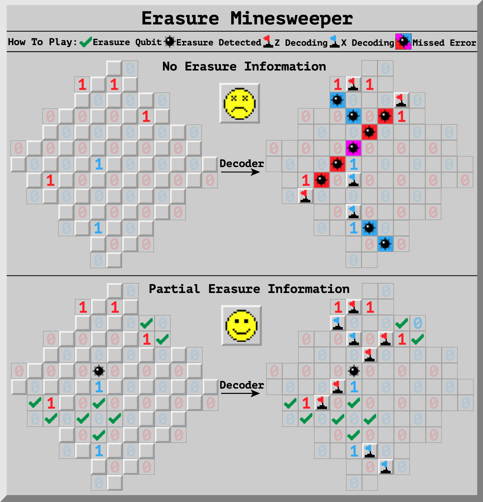
Figure 1. Viewing a hybrid-erasure architecture as a game of Minesweeper. Top: In a standard surface code, we receive syndrome bits (red and blue 1s) indicating that an error string terminates nearby. The decoder must find a valid explanation (red and blue flags) based only on this information. If the decoder guesses wrong, a logical error can occur. Bottom: When data qubits are erasure qubits, we gain extra information before decoding (black bombs and green checks on left) that help us decide which error string to predict, avoiding logical errors and achieving better error suppression. Middle: Partial improvements over error suppression persists when a carefully selected a subset of qubits are erasure qubits.
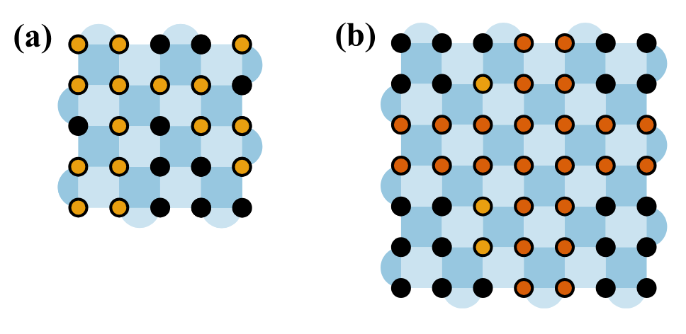
Figure 4. Examples of hybrid-erasure architecture. (a) \(\mathcal{A}(5,0.6,P_r)\) where the placement \(P_r = \{1,2,5,...,22\}\) is sampled at random. (b) \(\mathcal{A}(7,0.57,P^*)\). Since \(f_e\times d^2 = 27.93\), only 27 erasures are allocated, with $24$ erasures placed in 2 rows/columns, and the remaining 3 placed greedily, all as close to the center as possible.
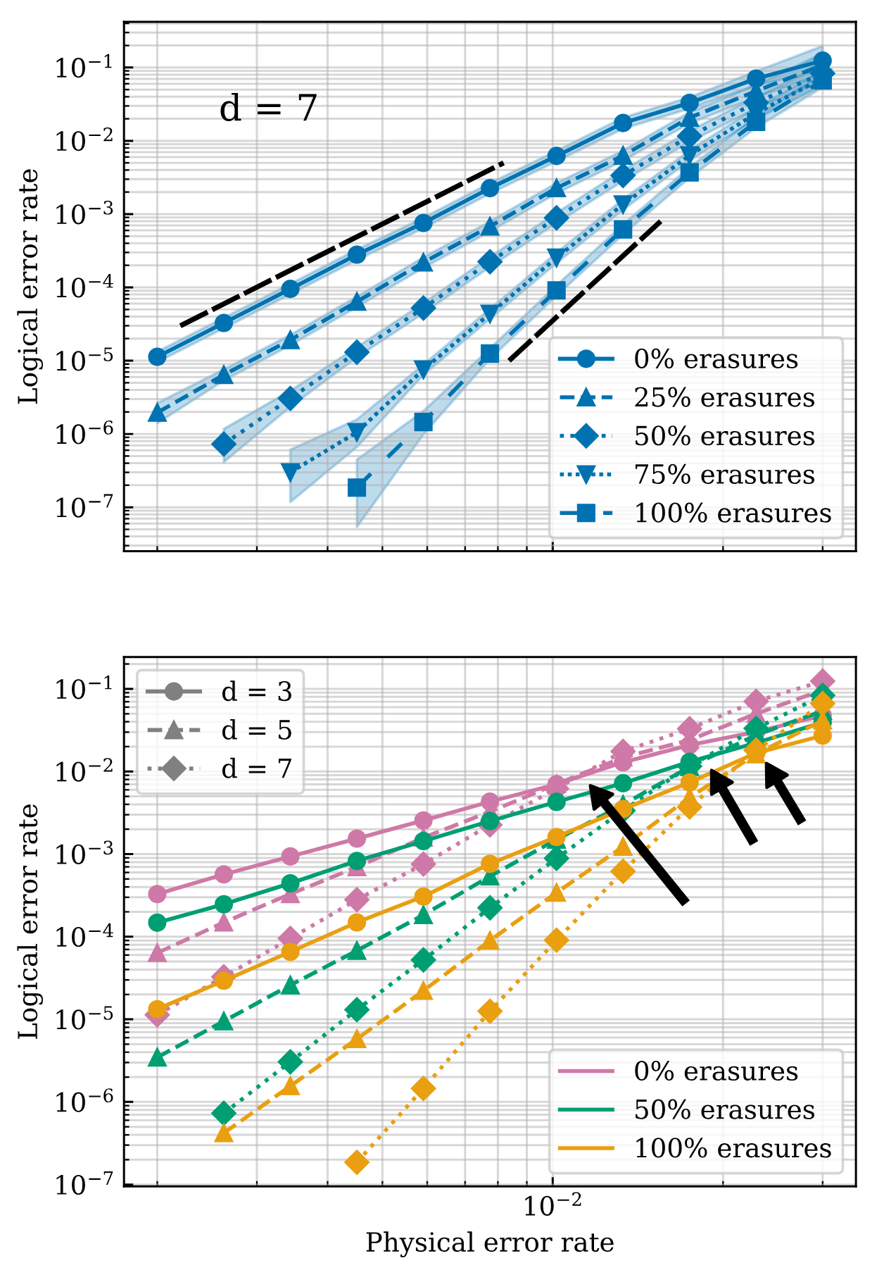
Figure 7. Logical memory performance of surface code of varying distance and varying fraction of erasure qubits, distributed according to our optimized heuristic. Top: For fixed code distance \(d=7\), increasing the fraction of erasure qubits improves \(d_\text{eff}\), evidenced by a steeper slope. Bottom: Increasing the fraction of erasure qubits also increases \(p_\text{th}\), the crossing point for different distances.
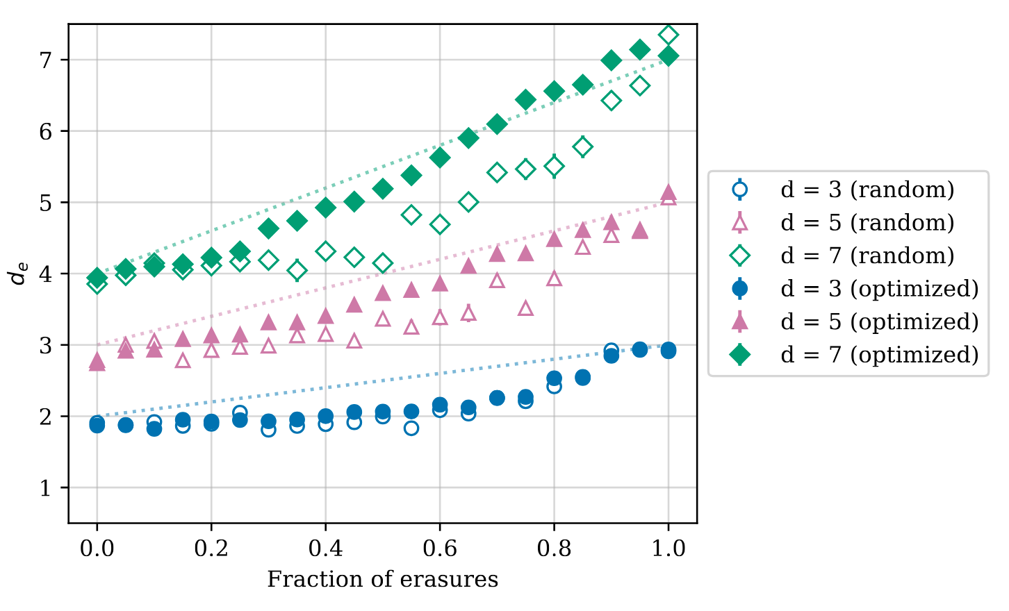
Figure 8. Effective distance \(d_\text{eff}\) of surface codes at various erasure qubit fractions. Optimized placement yields higher effective distance for intermediate erasure fractions. Lines show linear interpolation between \((d+1)/2\) and \(d\).
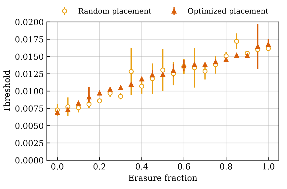
Figure 9. Extracted surface code thresholds for random and optimized placement for different erasure fractions. Optimized placement leads to more consistent improvements in threshold.
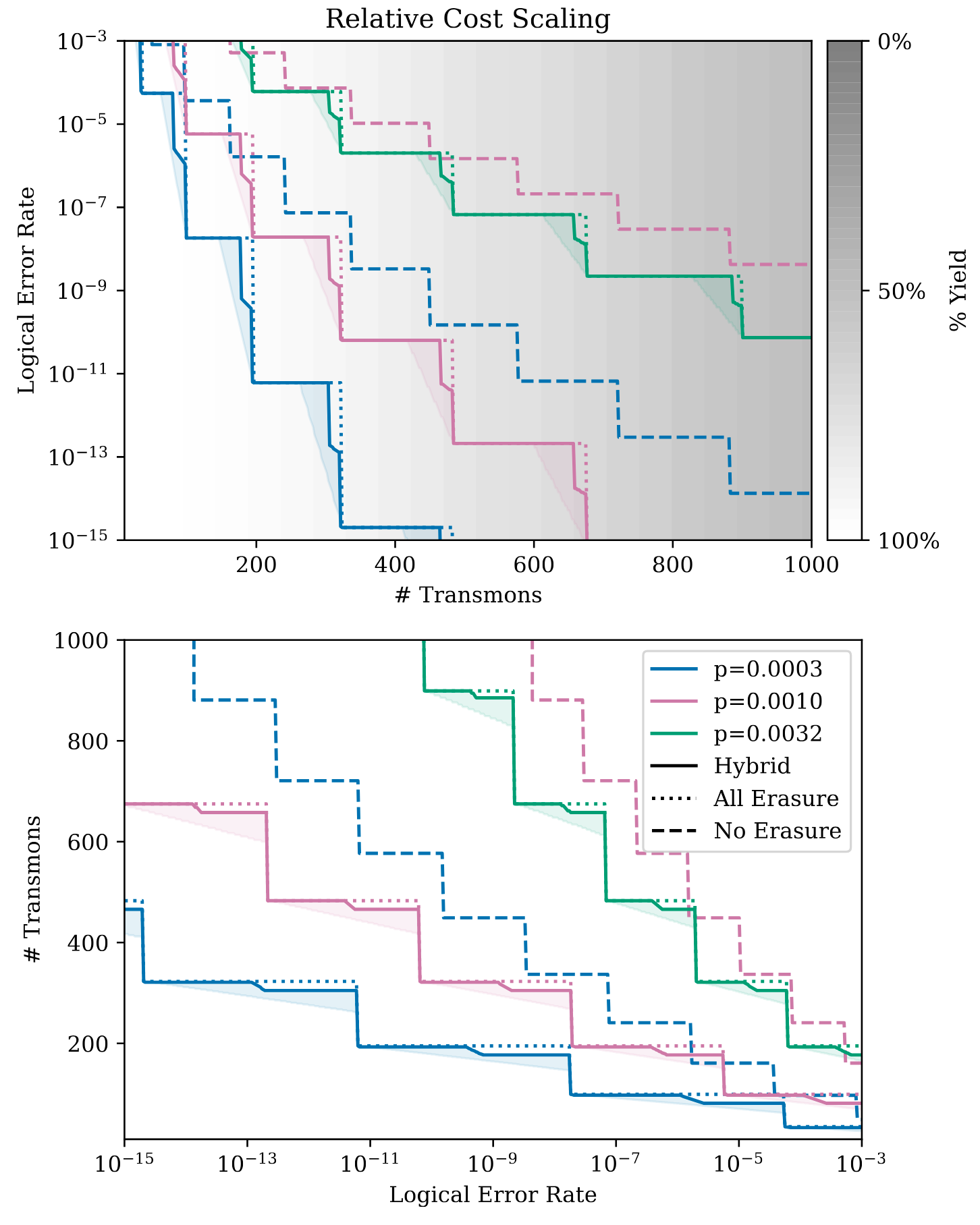
Figure 12. Scaling of costs in Figure 10 for larger systems using an all erasure architecture, a no erasure architecture, or a hybrid erasure architecture. All hybrid points sweep over and select the best erasure fraction. Shaded region represents area of possible hybrid erasure values in between analytical upper bound and approximate observed circuit-level lower bound. Top: Minimum possible logical error rate for fixed transmon cost. Background gradient indicates resulting single chip yield for a defect rate of \(10^{-3}\). Bottom: Minimum possible number of transmons for a target logical error rate.
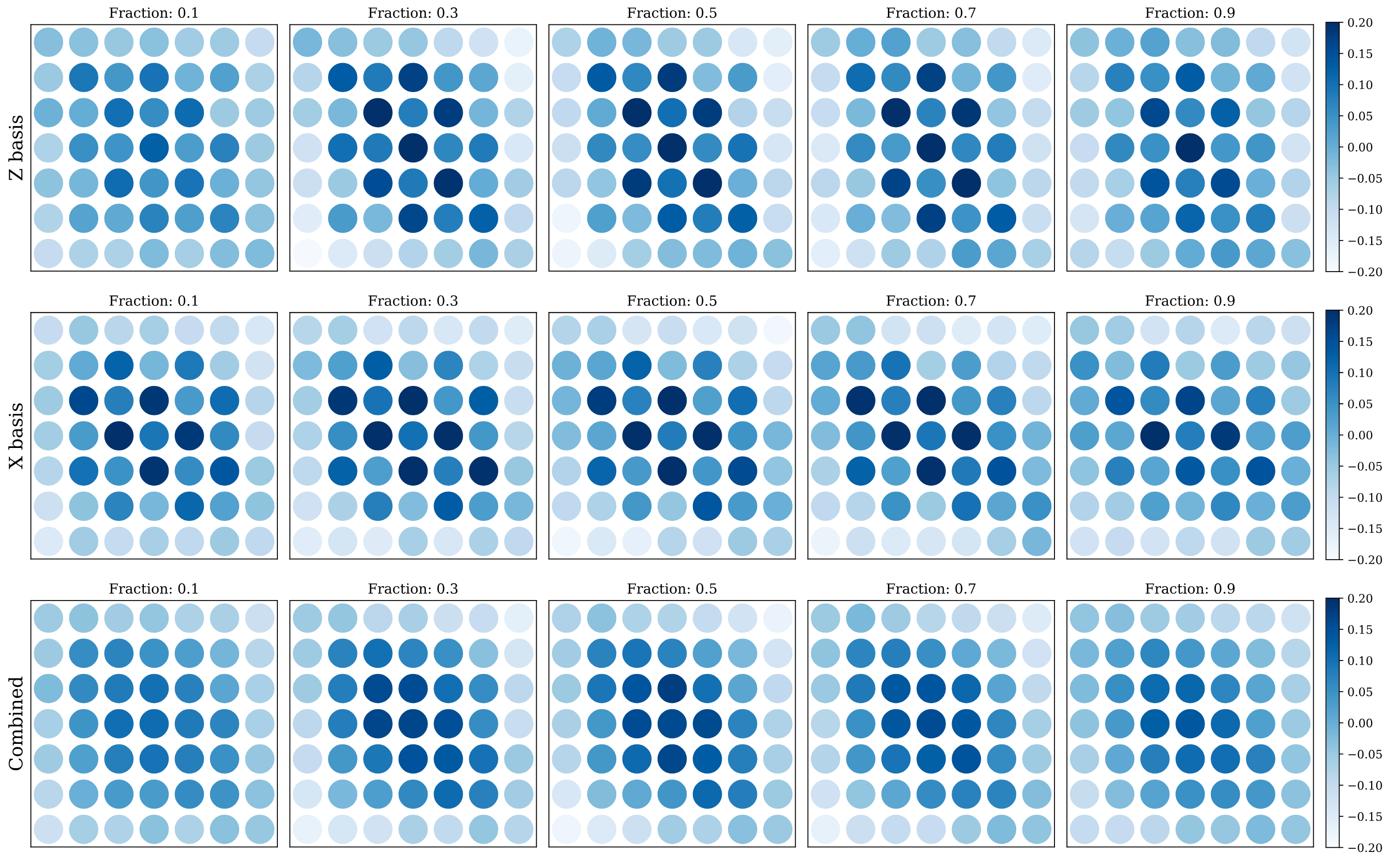
Figure 13. Effect of spatial placement of erasure qubits in a \(d=7\) surface code. Color indicates correlation between logical error rate and presence of an erasure qubit at each location in the \(7 \times 7\) grid of data qubits. Correlations are shown for \(\bar Z\) (top), \(\bar X\) (middle) and combined (bottom) error rates. “Checkerboard” patterns are evident in \(\bar Z\) and \(\bar X\) data but disappear for combined data.
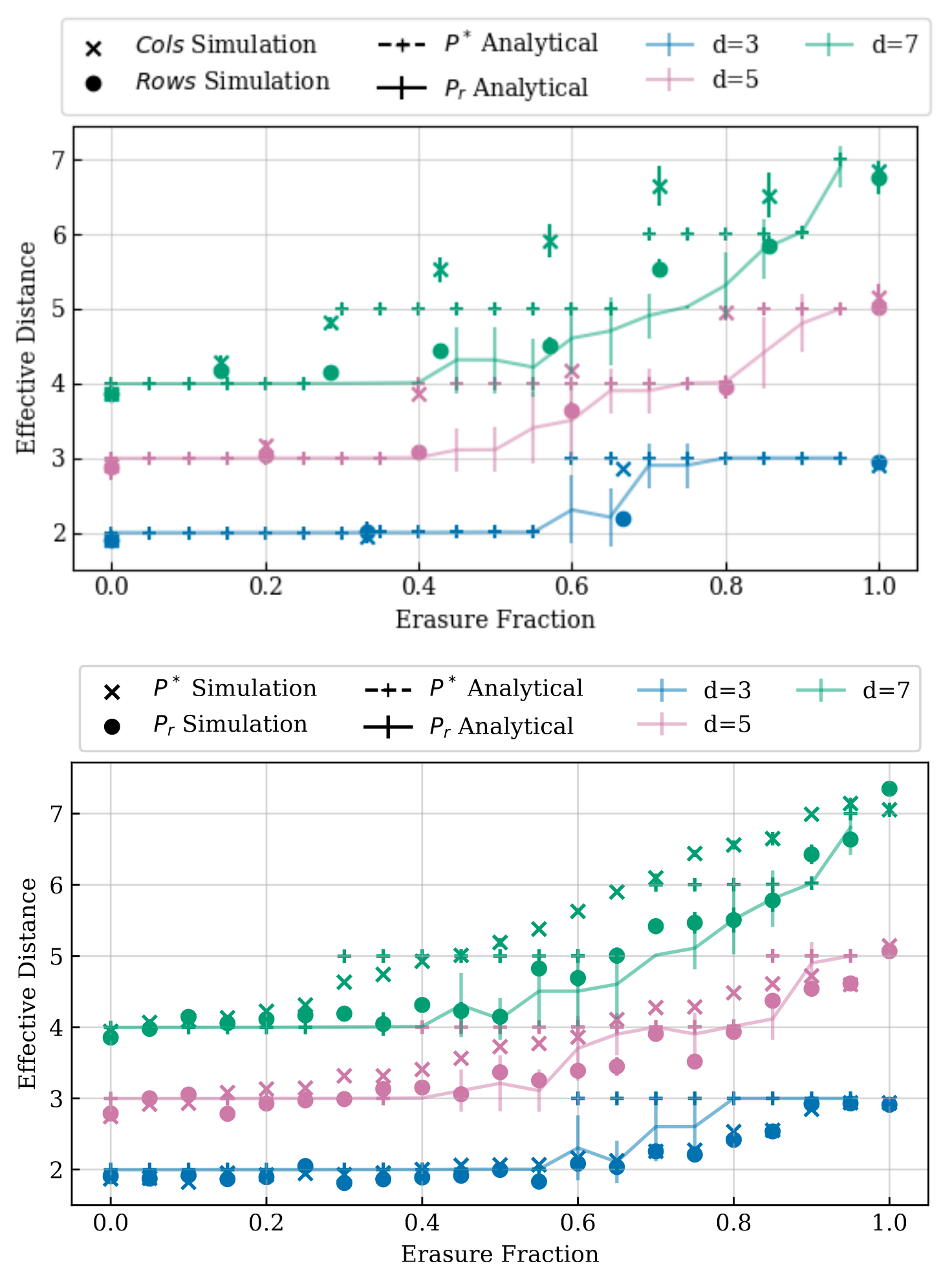
Figure 17. Comparing code-capacity model from Section III with simulation data from Section V for two different placement strategies (random placement \(P_r\), optimized heuristic \(P^*\)) and placements in consecutive rows and columns.
My Contributions
← back to jason-chadwick.com