Efficient control pulses for continuous quantum gate families through coordinated re-optimization
IEEE International Conference on Quantum Computing and Engineering (QCE 2023)
University of Chicago
University of Chicago
University of Chicago
University of Chicago
University of Chicago
University of Chicago
Abstract
We present a general method to quickly generate high-fidelity control pulses for any continuously-parameterized set of quantum gates after calibrating a small number of reference pulses. We find that interpolating between optimized control pulses for different quantum operations does not immediately yield a high-fidelity intermediate operation. To solve this problem, we propose a method to optimize control pulses specifically to provide good interpolations. We pick several reference operations in the gate family of interest and optimize pulses that implement these operations, then iteratively re-optimize the pulses to guide their shapes to be similar for operations that are closely related. Once this set of reference pulses is calibrated, we can use a straightforward linear interpolation method to instantly obtain high-fidelity pulses for arbitrary gates in the continuous operation space.
We demonstrate this procedure on the three-parameter Cartan decomposition of two-qubit gates to obtain control pulses for any arbitrary two-qubit gate (up to single-qubit operations) with consistently high fidelity. Compared to previous neural network approaches, the method is 7.7x more computationally efficient to calibrate the pulse space for the set of all single-qubit gates. Our technique generalizes to any number of gate parameters and could easily be used with advanced pulse optimization algorithms to allow for better translation from simulation to experiment.
[.pdf] [publication] [arXiv] [poster] [code]Selected Figures
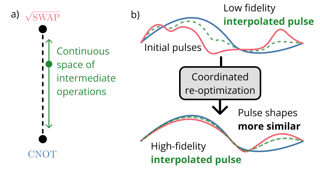
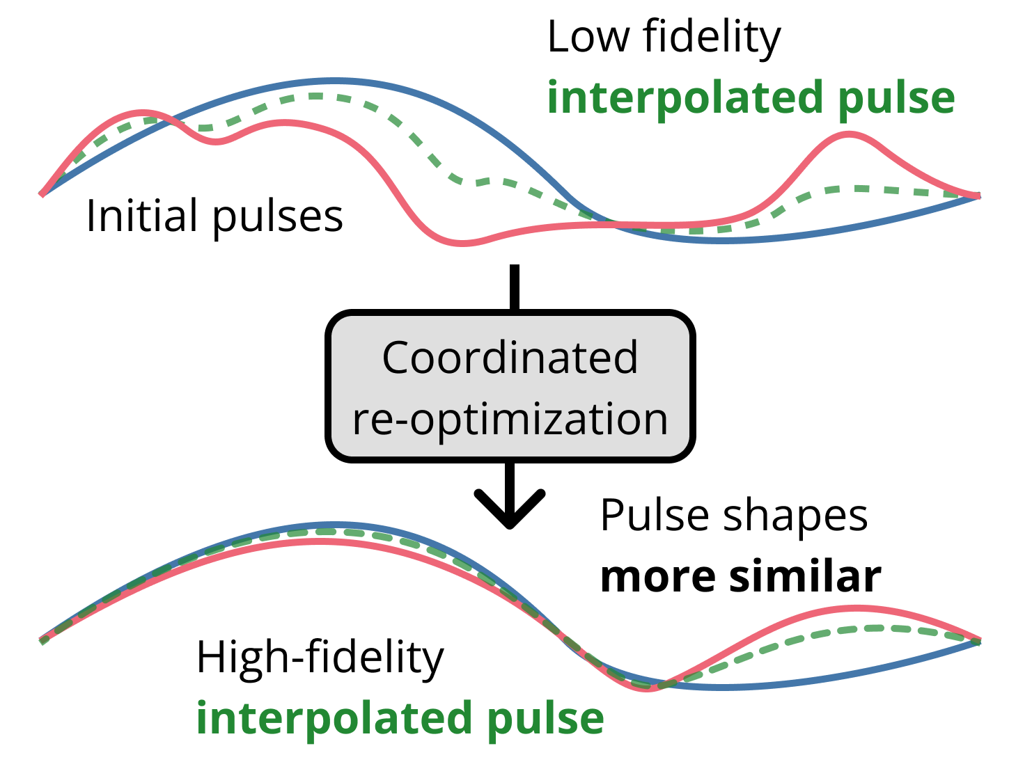
Figure 1. a) We seek to efficiently generate high-fidelity control pulses for continuous families of quantum gates. Here, we envision some continuous set of unitary operations between the $CNOT$ and $\sqrt{SWAP}$ operations. The goal is to efficiently obtain control pulses for any arbitrary point in this one-dimensional space of operations while only explicitly calibrating pulses at the two endpoints. b) Top: Consider some high-fidelity control pulses that implement $CNOT$ and $\sqrt{SWAP}$ (blue and red). We attempt to obtain a pulse for an intermediate operation (green) through linear interpolation. We find that interpolation yields poor results when the fixed pulses have very different shapes. Bottom: However, if we can re-optimize the pulses for $CNOT$ and $\sqrt{SWAP}$ to be more similar to each other (while still performing the correct operations), our simple linear interpolation method can obtain a high-fidelity pulse for the intermediate operation. Our methods generalize to higher-dimensional parameter spaces.
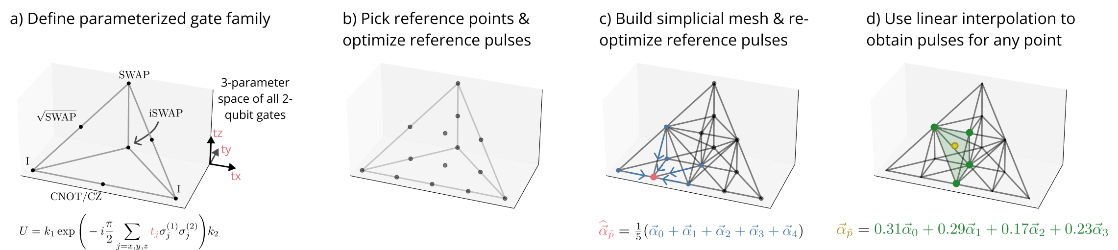
Figure 2. Overview of the example of our method provided in this work. More details on this specific example are provided in Section V. a) We use the Cartan decomposition (6) to define a three-dimensional space that contains all two-qubit operations. Our goal is to efficiently generate pulses for any arbitrary point within this continuous space. b) We choose several reference operations within the space and generate control pulses that implement these operations via optimal control software. Interpolating between these reference pulses does not necessarily provide a high-quality pulse immediately. c) To solve this problem, we iteratively re-optimize each reference pulse to be more similar to the average of nearby reference pulses, a process we call neighbor-average re-optimization. This process is described in Section II. d) Once these reference pulses have been fully calibrated, we can instantly obtain control pulses for any operation in the continuous family by performing linear interpolation between the nearest reference pulses. This process is described in more detail in Section III.
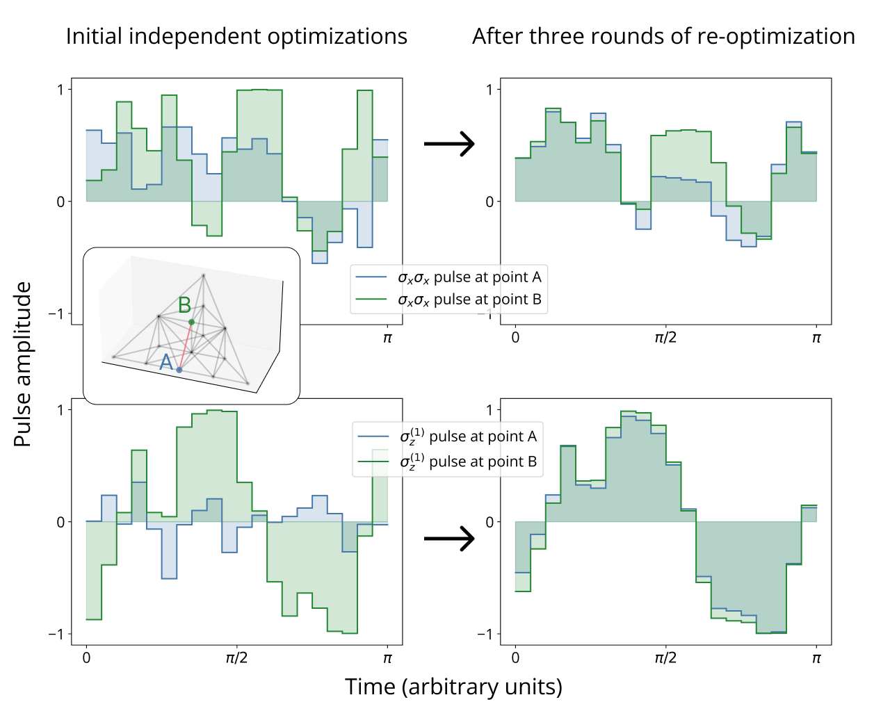
Figure 3. Comparison of pulse shapes for two adjacent reference points before and after several rounds of re-optimization. Point A corresponds to Cartan coordinates $(\frac 1 2, 0, 0)$ (the coordinates of $CNOT$ and $CZ$) and point B corresponds to coordinates $(\frac 1 2, \frac 1 4, \frac 1 4)$. Optimized controls for the two operations (from the same results as shown in Figure 4) are shown for the $\sigma_x \sigma_x$ control (top) and $\sigma_z^{(1)}$ control (bottom) of the Hamiltonian (6). Inset: locations of points A and B in the Weyl chamber. Left: the pulse shapes are initially significantly different between points A and B. Right: the pulses become far more similar after re-optimization, making interpolation easier, but still retain certain differences in their shapes that account for the differences in the resulting operations.
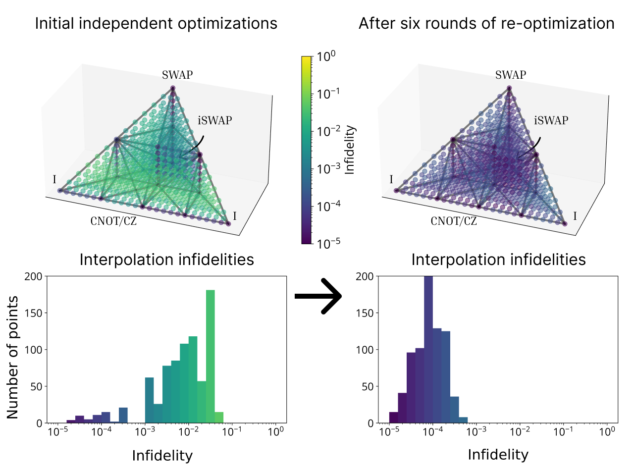
Figure 4. Interpolation quality after applying the re-optimization scheme. Axes on the top plots correspond to the three Cartan coordinates of two-qubit gates. Reference pulses are generated by optimal control software for 14 reference points in parameter space. Pulses for any point in the chamber can be obtained by linear interpolation between reference pulses. Left: interpolated pulse infidelities at 819 test points (granularity 1/24) after initial optimization of reference points. Black lines connect reference points and define the simplicial mesh that is used for interpolation. Each colored point represents a unitary operation defined by its coordinates. The color of each point is the infidelity of the pulse that is obtained via interpolation. Mean infidelity is $1.3 \pm 1.2 \times 10^{-2}$. Right: results after repeatedly re-optimizing each reference point to be near the average of its neighbors. Mean infidelity is improved to $1.0 \pm 0.8 \times 10^{-4}$.
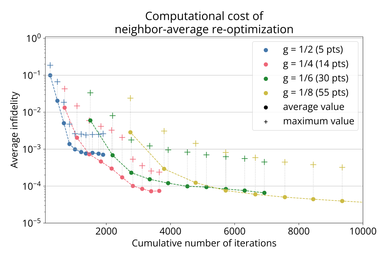
Figure 5. Different reference point granularities translate to varying amounts of classical computation time needed to optimize all reference pulses. Consecutive points with the same granularity $g$ correspond to subsequent re-optimization rounds, which can further improve average (and maximum) infidelity at the cost of more optimizer iterations. Each optimization iteration corresponds to one system evolution. The points indicated by the plus sign indicate the worst infidelity of any test point.
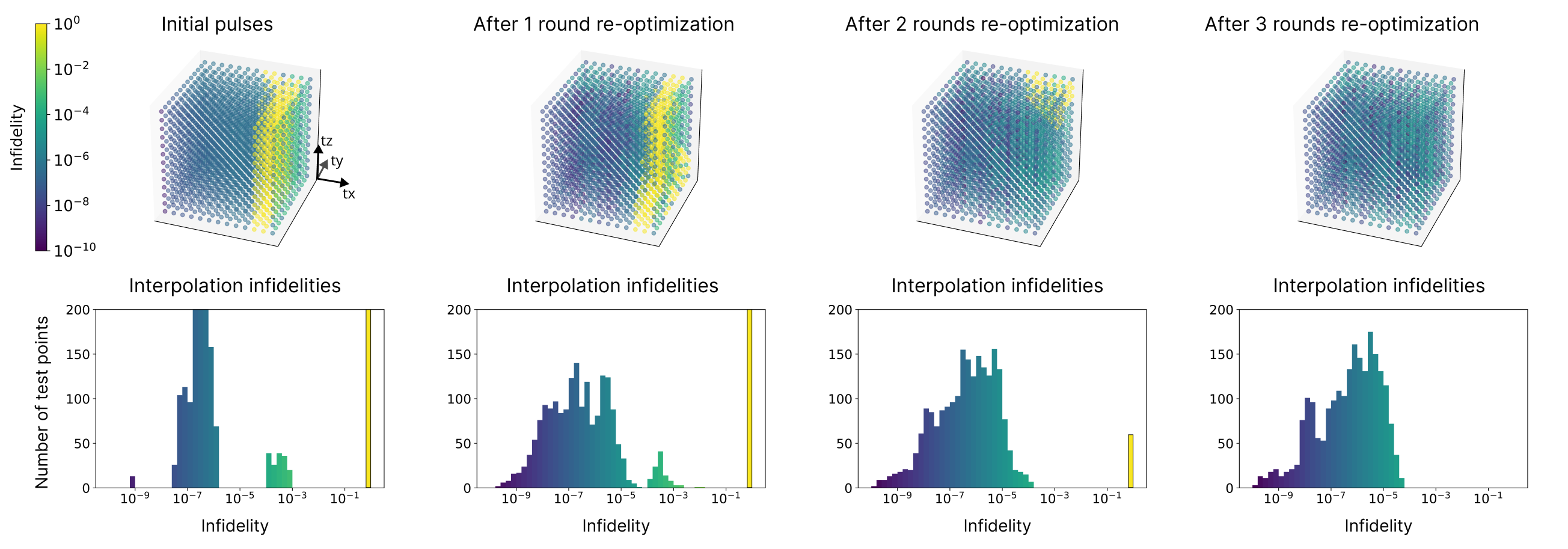
Figure 6. Infidelities at 2197 test points within the parameter space of single-qubit rotations (see Equation (9)). Average and worst-case infidelities are shown in Table I. We observe a region of extremely poor interpolation quality (yellow), indicating that the pulses on either side of this area have very different shapes and actions. Intuitively, the pulses on the two different sides of this boundary take different routes around the Bloch sphere to reach the target unitary. Subsequent rounds of neighbor-average re-optimization reduce the size of this poor interpolation region and eventually eliminate it, resulting in an average interpolation infidelity (across all test points) of $3.5 \pm 6.6 \times 10^{-6}$ after three rounds of re-optimization.
My Contributions
← back to jason-chadwick.com